Parallel Computing Techniques

This project is done as part of a course Advanced Computing Systems (EE4C07) at Delft University of Technology

Tools used: C++, C++ STL, GProf, GNU Compiler, CMake, OpenMP, OpenCL, CUDA, NVProf

Project source: https://gitlab.com/nvn3/acs—lab

Contributing member:

Task 1/3: Matrix Multiplication three implementation

The goal of this task is to explore different parallel programming techniques and benchmark their speed up. We use vector inner product and traditional matrix multiplication method to perform the benchmarks in three different constructs:

1. Single Instruction Multiple Data (SIMD)
2. OpenMP
3. OpenCL

Benchmark details

The time consumed shown in this section is a result of running each trail three times. The benchmarking is done on datatypes double and float.

Vector Inner Product

For vectors of dimensions A(1xN) and B(Nx1), the vector product consists of N multiplication and N-1 addition operations. Figure . shows the increase in time with the increase in size for both the datatypes.

Matrix Multiplication

For given matrices A and B, serial method ses multiple loops to fetch the right elements from each matrix and performs element-wise multiplication. In addition to that, it uses another loop to perform addition to calculate an element in the result. For two matrices A (MxK) and B (KxN), to obtain the result C (MxN), it performs M.N.K number of multiplications and M.N.(K-1) number of additions.

A conventional serial implementation can benefit from parallelism. The subsequent section shows how the computation time is decreased with each of the parallel constructs.

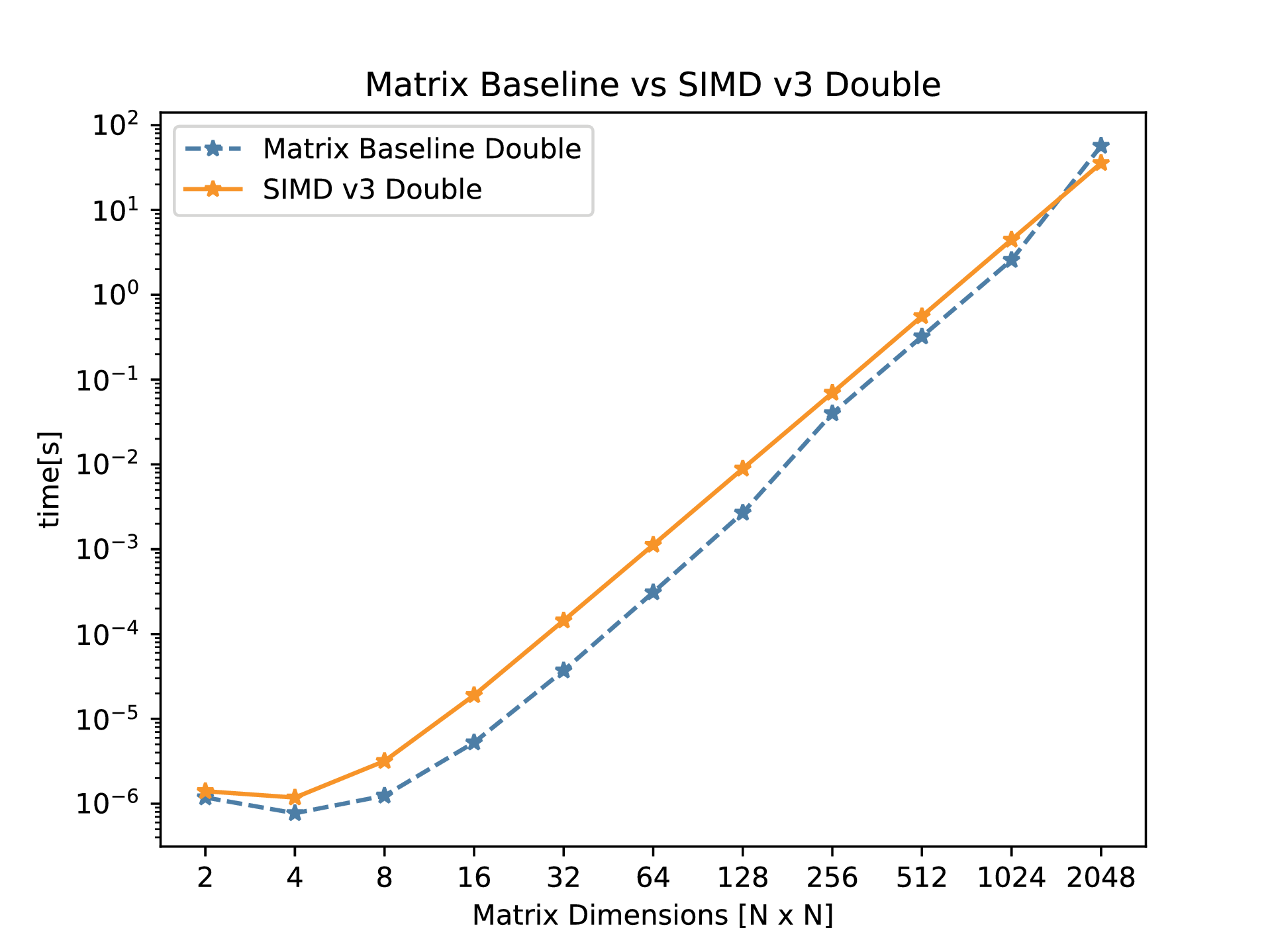
SIMD Extensions

SIMD extensions are supported on Intel and ARM in the form of AVX and Neon respectively. In this discussion we stick to Intel’s AVX (Advanced Vector eXtensions).

As the name suggests, SIMD can perform an arithmetic operation on multiple data in a single clock cycle. Depending on the AVX version present in the processor, the size of the AVX registers vary. For the experiments performed in this post, AVX-256 version, in which the registers are 256 bits, is used. The number of data elements that fit into the register depends on the data type. For example, 8 float elements or 4 double elements can fit into an AVX-256 register.

The following are the steps taken:

1. To achieve a speed up, the rows of the first matrix and columns of the second matrix are loaded into two separate AVX registers and use SIMD instructions to perform multiplication. This step is a major speed up in this technique. While the multiplication got faster with the implementation of SIMD, the horizontal addition would still remain the bottleneck in the performance. This step alone didn’t account for a major speed-up.

2. After profiling further, it was found that the time taken to load the data into the registers is one of the bottleneck. The row of first matrix is loaded into the first vector and remain until the all the columns are multiplied. By doing this, a significant improvement was observed.

3. To improve upon this furhter, we have identified another bottleneck which is to be the horizontal additions. This was again achieved with vector horizontal additions. This replaces another step in the iteration.

The final benchmarks are shown below:

OpenMP

OpenMP is a very simple and practical technique to implement parallelism to a program. It instructs a given number of threads to work in parallel on a specified part of a program. This is known as multithreading, where the master thread forks off into multiple threads to execute that particular piece in parallel [todo-ref]. This method yields faster run times compared to serial executions of the same task. OpenMP commands are invoked by pragmas in the code and a clause. The implementation of OpenMP uses for loops which perform matrix multiplication analytically. That is, the outer most loop keeps track of the row of the A matrix, the middle loop tracks the columns of matrix B, and the inner most goes through the current column of A and current row of B. With some basic math we are able to compute the resulting matrix. Parallelizing the for-loop can be done with the following pragma:

#pragma omp for

We immediately saw the performance increase of using OpenMP compared withe the baseline matrix multiplication. Additionally, it was noticed that the difference between using 4 and 8 threads were slim for low sized matrices. However, for bigger matrices the performance of using 8 threads was significantly greater.

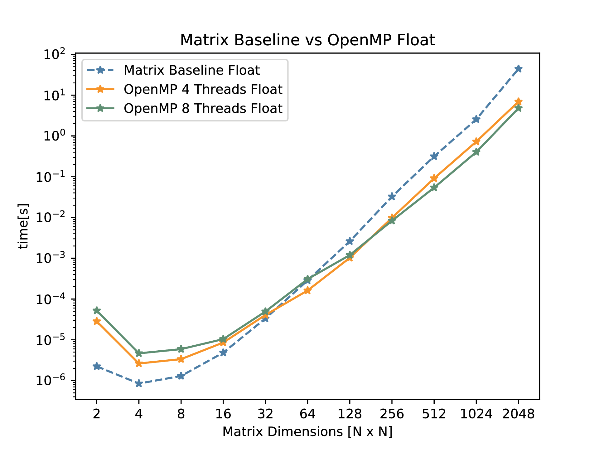
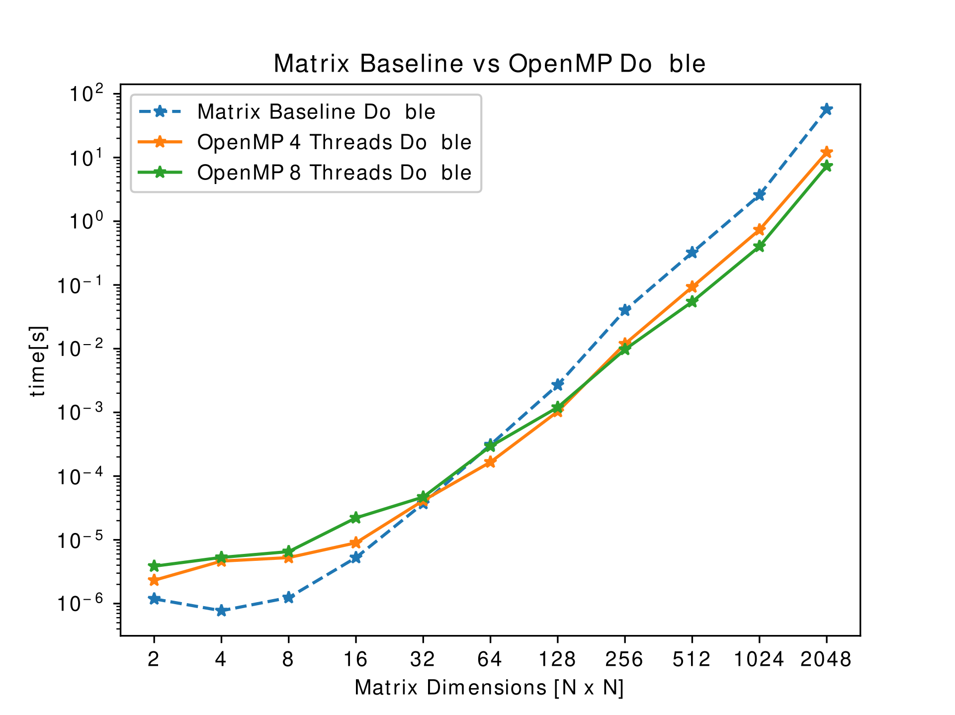
The results obtained don’t adhere to Amdhal’s law mainly because of the cache misses when the work is split among multiple cores.

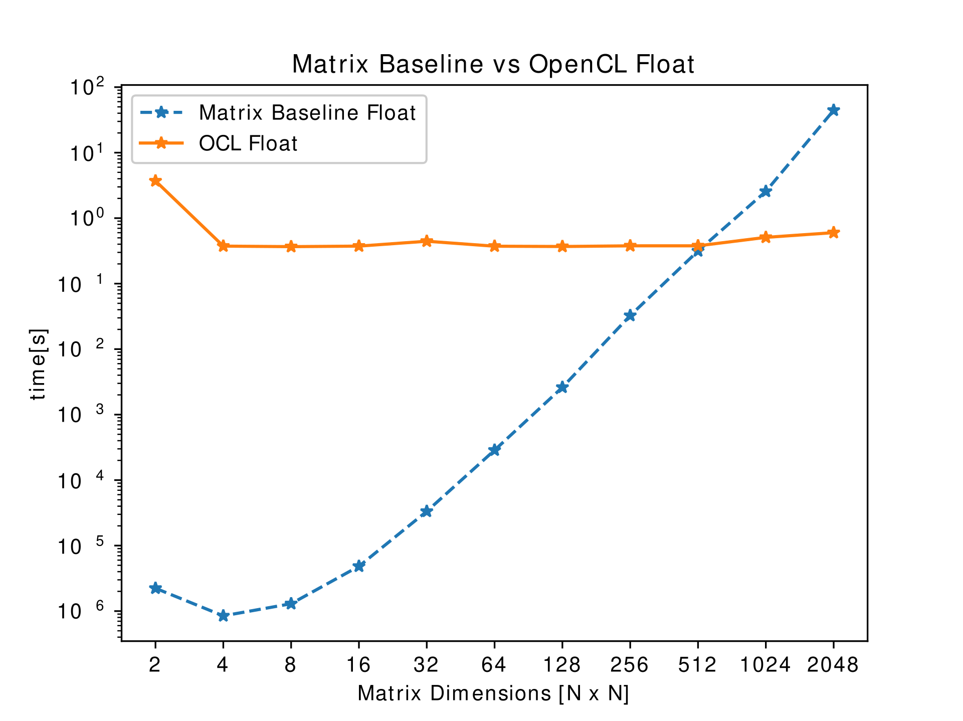
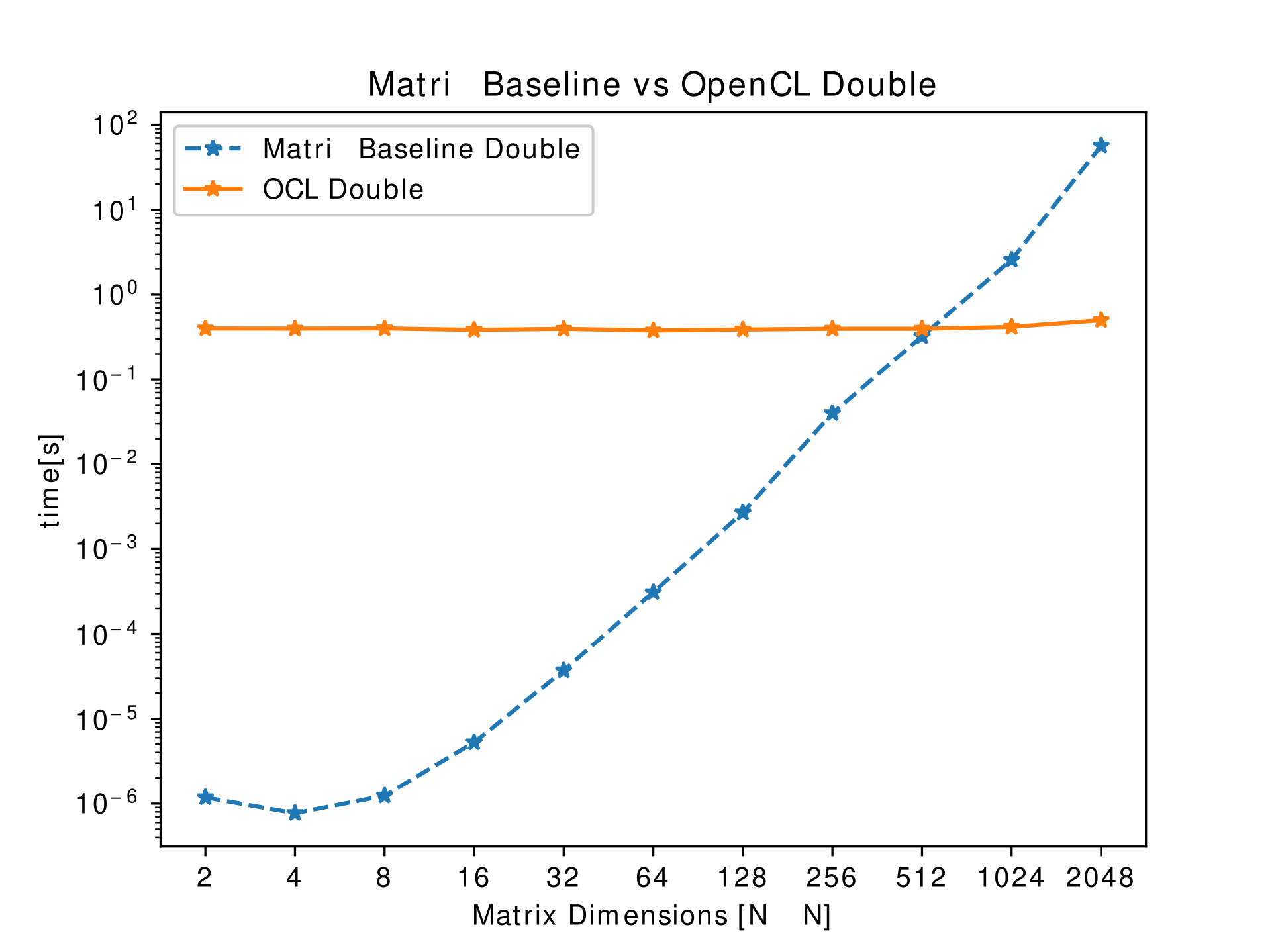
OpenCL

OpenCL is a framework which enables the writing of programs that can be executed on heterogeneous architectures, such as CPUs, GPUs, FPGAs and DSPs. It provides robust API for parallel computing featuring both instruction and data-level parallelism.

The results yielded with this implementation were remarkable, in which the serial implementation on the CPU was turned into a parallel implementation on the GPU. Each of the parallel job (know as a work-item) that needs to be executed are handed over to a GPU core. In OpenCL, the kernel is the code that is put in the form of a work-item on the GPU cores. Each of the loop is assigned to an independent work-item.

While the expected speed-up is proportional to the number of GPU cores, the observation was rather counter-intuitive. The main reason for the slow-down is the overhead of the memory transactions. This slow-down because of the overhead is noted for smaller matrices.

Task 2/3: Image Processing Algorithms Speed-up

This task explores the usage of CUDA to manipulate images using some basic image processing algorithms. The four image processing algorithms implemented in this task are:

1. Histogram Calculation
2. Contrast Enhancement
3. Ripple Effect
4. Gaussian Blur

Benchmark details

The above image processing algorithms are performed on five different images with varying pixel count: 25, 5,184, 16,384, 108,032, 262,144 and 12,000,000.

Histogram Calculation

Extracting the histogram of images is the first step of the image processing pipeline. Its results are later used in other processing algorithms. This algorithm calculates the total intensity of the image’s pixels for each one of the channels (RGBA color space). The baseline implementation is a serial algorithm which traverses through each of the pixel and finds the intensity of each channel in that pixel.

Each of the loop in serial implementation is unrolled and each of the pixel is given as a work-item to each CUDA thread. The speed-up is seen only for larger images.

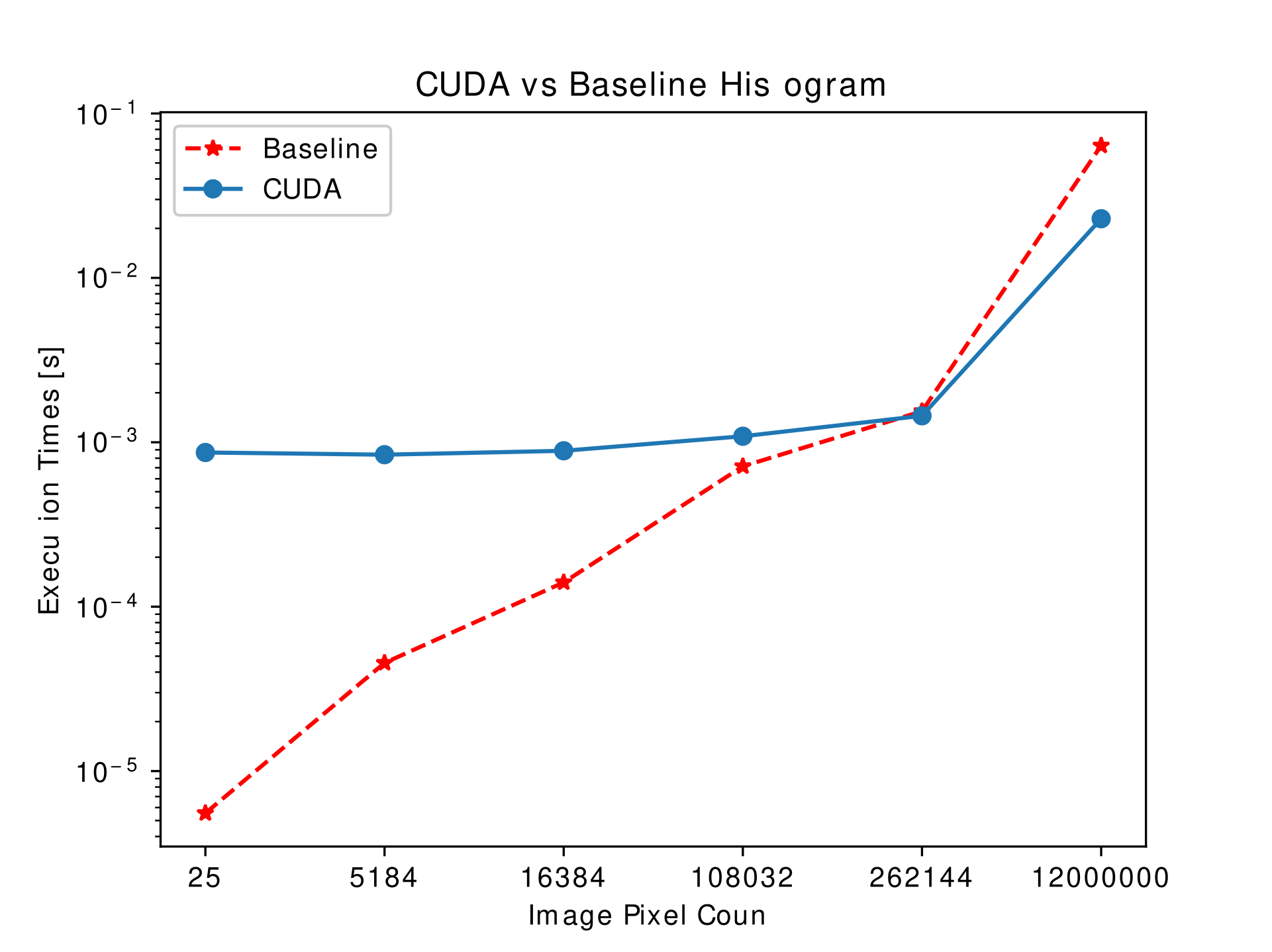
Since histogram has less arithmetic intensity as shown in the following figure, the improvement achieved is low or very much same as the serial implementation for larger images. Another bottleneck with the CUDA implementation is that the reduce function needs to synchronize with other threads inorder to calculate the final sum of the channel intensity.

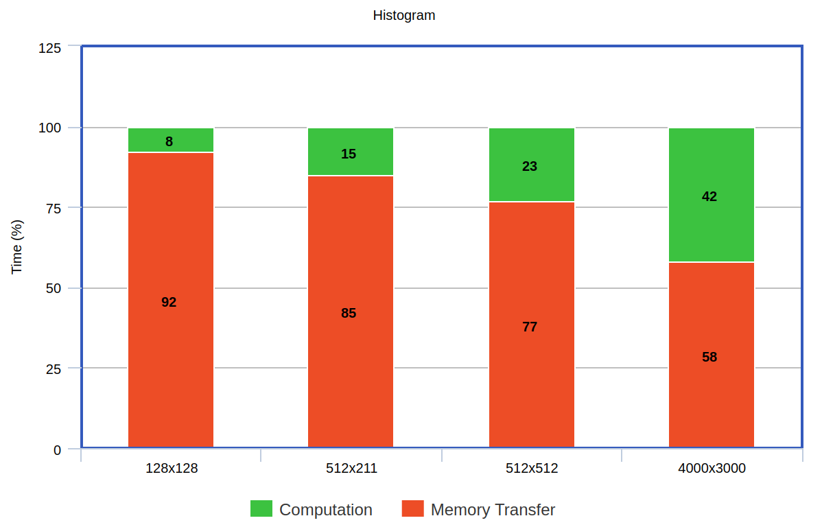
A significant speed-up is not seen because the overall time taken is dominated by the memory transaction.

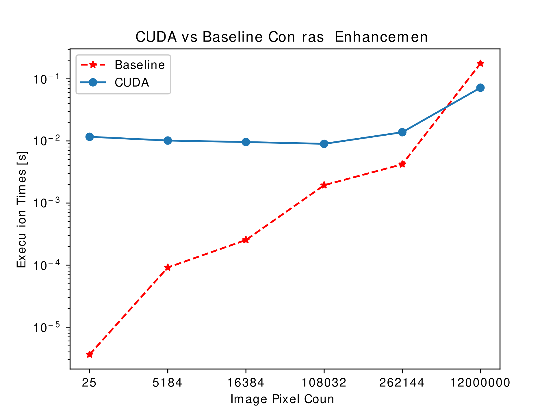
Contrast Enhancement

Contrast enhancement is done to make the image appear more vivid and clear. This is achieve by normalizing the histogram produced in the previous step. By applying this, we expand those values over a wider range, thereby covering a larger color spectrum.

This processing is done in a way similar to the previous case. Each of the pixel’s processing is pushed to each of the GPU core. To that effect, when this is done independently, the result observed is very similar to the one obtained in case of histogram calculation which is shown in the figure below. However, a considering the stage where this image processing needs to be done, a huge speed-up can be gained by storing the histogram of the image and the image on the GPU itself (as long as there is enough memory).

Ripple Effect

Gaussian Blur

Task 3/3: K-Nearest Neighbours Algorithm Speed-up

Verdict: As it can be observed, using SIMD doesn’t give the highest performance gain. Despite that being the case, SIMD neither needs multiple cores nor any expensive hardware additions. SIMD takes the advantage of the ISA.

Written on September 17, 2018